module aicafe.img

This module contains functions for image processing.

cummul_mats(mats)

Compute cumulative multiplications of matrixes.

Parameters:

Name	Type	Description	Default
mats	ArrayLike	Shape of [P, N, N], a group of \(N\times N\) matrixes.	required

Returns:

Name	Type	Description
mats_cum	NDArray	Shape of [P, N, N]. mats_cum[i] represents \(A_iA_{i-1}\cdots A_0\), where \(A_i\) is the matrix represented by rots[i].

distance(vecs1, vecs2)

Compute the distances between two group of vectors. Both inputs must be able to be broadcast together.

Parameters:

Name	Type	Description	Default
vecs1	ArrayLike	Shape [..., 3], an array of 3D coordinates.	required
vecs2	ArrayLike	Shape [..., 3], an array of 3D coordinates.	required

Returns:

Type	Description
NDArray	Array with broadcast shape. E.g., with vecs1's shape [A, 1, 3] and vecs2's shape [1, B, 3], the result's shape will be [A, B].

distance2d(vecs1, vecs2)

Compute the distances between two group of vectors after projecting them to the x-y plane, i.e., the z coordinate will be regarded as 0. Both inputs must be able to be broadcast together.

Parameters:

Name	Type	Description	Default
vecs1	ArrayLike	Shape [..., 3], an array of 3D coordinates.	required
vecs2	ArrayLike	Shape [..., 3], an array of 3D coordinates.	required

Returns:

Type	Description
NDArray	Array with broadcast shape. E.g., with vecs1's shape [A, 1, 3] and vecs2's shape [1, B, 3], the result's shape will be [A, B].

grids_polar_from_bases(uvs, n_points_dia=100, n_angles=120)

Generate polar grids of points from 2D basis vector pairs.

Specifically, let \(u_k,v_k\) be the \(k\)-th pair of basis vectors (parallel to x and y axes, respectively), \(T\) be the numbers of angles/diameters, and \(R\) be the number of points on each diameter. The origin is located at the center of the grid, so the point in the \(i\)-th row and \(j\)-th column of the \(k\)-th grid (\(0\leqslant i \leqslant T-1,0\leqslant j \leqslant R-1\)) is

\[ p_{ij}^k=(i-\frac{R-1}{2})[\cos (\frac{2\pi}{T-1}j)u_k+\sin (\frac{2\pi}{T-1}j)v_k] \]

The point coordinates of the resulting grids.

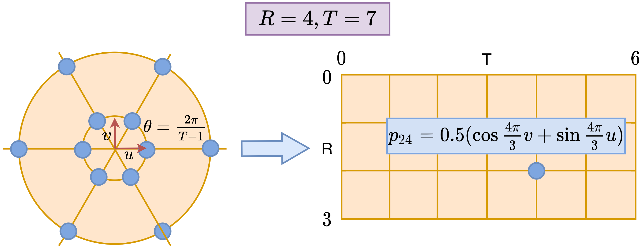
Parameters:

Name	Type	Description	Default
uvs	ArrayLike	Shape of [P, 2, 3]. uvs[k-1, 0] represents \(u_k\), and uvs[k-1, 1] represents \(v_k\).	required
n_points_dia	int	The number of points on each diameter.	100
n_angles	int	The number of angles/diameters.	120

Returns:

Name	Type	Description
grids	NDArray	Shape of [P, R, T, 3]. grids[k, i, j] represents \(p_{i,j}^k\), the point in the \(i\)-th row and \(j\)-th column of the \(k\)-th grid.

grids_rect_from_bases(uvs, n_rows=200, n_cols=200, loc_ori='lower_left')

Generate rectangular (Cartesian) grids of points from 2D basis vector pairs.

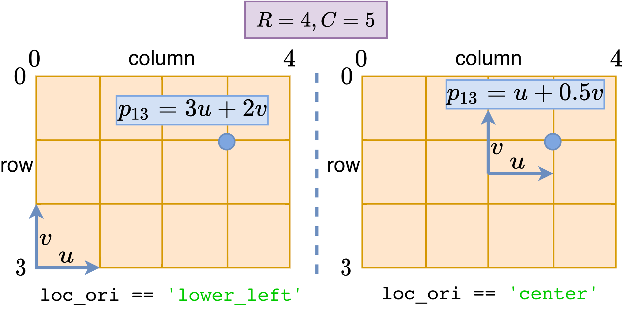
Specifically, let \(u_k,v_k\) be the \(k\)-th pair of basis vectors (parallel to \(x\) and \(y\) axes, respectively), and \(R,C\) be the numbers of grid rows and columns, respectively, thus \(0\leqslant i\leqslant R-1,0\leqslant j\leqslant C-1\).

• If the origin is located at the lower-left corner of the grid, i.e., loc_ori=='lower_left', then the point in the \(i\)-th row and \(j\)-th column of the \(k\)-th grid is

\[ p_{ij}^k=ju_k+(R-i-1)v_k, \]

• If the original is located at the center of the grid, i.e., loc_ori=='center', then

\[ p_{ij}^k=(j-\frac{C-1}{2})u_k+(\frac{R-1}{2}-i)v_k. \]

The point coordinates of the resulting grids with different loc_ori.

Parameters:

Name	Type	Description	Default
uvs	ArrayLike	Shape of [P, 2, 3]. uvs[k-1, 0] represents \(u_k\), and uvs[k-1, 1] represents \(v_k\).	required
n_rows	int	The number of rows of each grid.	200
n_cols	int	The number of columns of each grid.	200
loc_ori	str	'lower_left' or 'center'. The location of the origin for each grid.	'lower_left'

Returns:

Name	Type	Description
grids	NDArray	Shape of [P, R, C, 3]. grids[k, i, j] represents \(p_{i,j}^k\), the point in the \(i\)-th row and \(j\)-th column of the \(k\)-th grid.

mats_rot(vecs1, vecs2)

Compute the rotation matrixes that rotate vectors in vecs1 to those in vecs2.

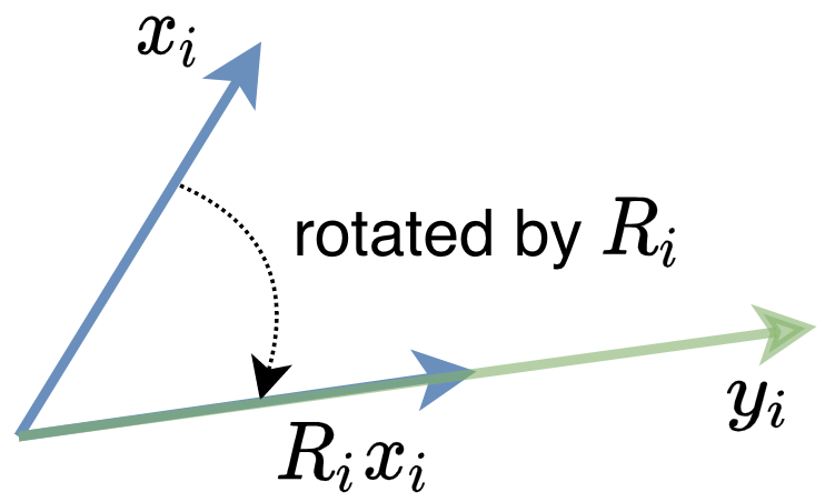
Specifically, let \(x_i\) be the \(i\)-th vector in vecs1, and \(y_i\) be the \(i\)-th vector in vecs2, and \(R_i\) is the \(i\)-th rotation matrix in the returned mats, then \(R_i\) is orthonormal, and \(R_i\frac{x_i}{\|x_i\|}=\frac{y_i}{\|y_i\|}\).

Parameters:

Name	Type	Description	Default
vecs1	ArrayLike	Shape [P, 3], an array of 3D coordinates.	required
vecs2	ArrayLike	Shape [P, 3], an array of 3D coordinates.	required

Returns:

Name	Type	Description
mats	NDArray	Shape of [P, 3, 3]. Array of rotation matrixes, where mats[i] is the rotation matrix that rotates vecs1[i] to vecs2[i], i.e., mats are orthonormal matrixes, and mats @ normalize(vecs1)[..., None] == normalize(vecs2)[..., None].

mod(vecs)

Compute the moduli of vectors.

Parameters:

Name	Type	Description	Default
vecs	ArrayLike	Shape [..., 3], an array of 3D coordinates.	required

Returns:

Type	Description
NDArray	Shape of [...].

normalize(vecs)

Normalize vectors to unit length.

Parameters:

Name	Type	Description	Default
vecs	ArrayLike	Shape of [..., 3], an array of 3D coordinates.	required

Returns:

Type	Description
NDArray	Shape of [..., 3], the normalized vectors, i.e., the L2 norms of last dimension are 1. If a vector in vecs has length of 0, then the normalized vector will still be a zero vector.

points_ori2xsec(points, curve)

Transform given points from original image space (in which the curve is localized) to the space of stacked cross-sectional images (which are generated from points on the curve).

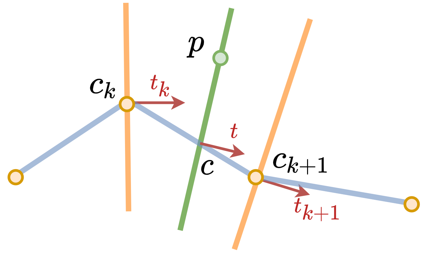
Specifically, let the points on the curve be \(\{c_k\}\), and \(t_k\) be the tangent vector of the curve at \(c_k\), then \(t_k\) is perpendicular to the cross-sectional plane \(\mathcal{S}_k\) through \(c_k\). Given a point \(p\) to be transformed, the algorithm first determines between which two planes \(\mathcal{S}_k,\mathcal{S}_{k+1}\) it lies, by asserting that the angle between \(\overrightarrow{pc_k}\) and \(\overrightarrow{pc_{k+1}}\) must be obtuse. There may be multiple \(k\)'s satisfying this condition, and the \(k\) with the minimal \(\|c_kp\|\) will be selected. If there is no \(k\) satisfying the condition, \(p\) is not valid for transformation, thus will be discarded, i.e., no transformed result of \(p\) will be included in the return array.

After determining \(k\), the \(z\)-coordinate of transformed \(p\) is \(k+1-\lambda\), where \(\lambda(p)\) is calculated by solving

\[ \left\{\begin{array}{l} c=\lambda c_{k}+(1-\lambda) c_{k+1} \\ t=\lambda t_{k}+(1-\lambda) t_{k+1} \\ \langle cp, t\rangle=0 \end{array}\right. \]

where \(t\) can be regarded as the norm vector of the cross-sectional plane \(\mathcal{S}\) that \(p\) lies in, and \(c\) is the intersection point of \(\mathcal{S}\) and \(c_kc_{k+1}\).

The \(x\)- and \(y\)-coordinates of transformed \(p\) are calculated as the projections of \(\overrightarrow{cp}\) on the two unit basis vectors \(u,v\) of \(\mathcal{S}\), where \(u,v\) are calculated using the algorithm described in aicafe.img.vecs_basis_xsec.

Parameters:

Name	Type	Description	Default
points	ArrayLike	Shape of [P, 3], 3D coordinates representing points in the original image space. These points are usually close to the curve.	required
curve	ArrayLike	Shape of [C, 3], 3D coordinates representing the points on the curve.	required

Returns:

Type	Description
NDArray	Shape of [P0, 3], 3D coordinates representing points in the cross-sectional image space, each of which corresponds to a point valid for transformation in points. P0 is the number of valid points.
list[int]	Shape of P0, indexes of points valid for transformation.

points_sur_curve(curve, box=None, rad=3)

Get the grid points surrounding a curve.

Parameters:

Name	Type	Description	Default
curve	ArrayLike	Shape of [P, 3] (\(P\geqslant 2\)), an array of 3D coordinates representing the points on the curve. The coordinates must be non-negative.	required
box	ArrayLike	Shape of [3], the bounding box containing the curve and the surrounding points. Note that the box always has a vertex of \((0,0,0)\), thus only 3 (rather than 6) parameters are needed. If None, it will be calculated as the smallest box that contains the curve.	None
rad	float	A point is surrounding the curve if and only if there exists a point on the curve such that the distance between the two points is less than or equal to radius.	3

Returns:

Type	Description
NDArray	Shape of [Q, 3], an array of 3D coordinates representing the grid points around the curve.

sample_array(array, points, mode_interp='linear', value_pad=0)

Sample/Interpolate values of an array at given points (locations).

Usually, the array represents an image, and the points represents a multi-dimensional grid of coordinates. Specifically, an image \(I:\Omega\rightarrow\mathbb{R}^C\) is regarded as a mapping (function) from the image space \(\Omega\subset\mathbb{R}^D\) to the space of pixel values, that is, \(D=2\) or \(3\) for a 2D or 3D image, and \(C=1\) or \(3\) for a grayscale or RGB image. Therefore, the input array contains sampled values of the image on a regular grid, and the input points contains \(D\)-dimensional coordinates where the pixel values need to be interpolated.

Parameters:

Name	Type	Description	Default
array	np.ndarray	Multi-dimensional. Typically, the shape is [B, X, Y] or [B, X, Y, Z] for a batch of 2D or 3D grayscale image; [B, 3, X, Y] or [B, 3, X, Y, Z] for a batch of 2D or 3D RGB images. The dimension of B is not needed if only one image is interpolated. Note that for grayscale images, there should not be a dimension with size 1 before X, due to Scipy's behavior (see the Notes of Scipy for more information).	required
points	ArrayLike	Shape of [..., n_dims], where n_dims is the dimension of array. For example, if shapes of array and 'points' are [B, X, Y] and [5, 7, 3], respectively, then points[i, j]==[b=2, 0.3, 0.4] means that the point \(p_{ij}\) is in the 0.3-th row and 0.4-th column of the \(b=2\)-nd image.	required
mode_interp	str	'linear' or 'nearest'. The mode of interpolation.	'linear'
value_pad	float	Interpolated value for points outside the array space \(\Omega\) (domain, coverage).	0

Returns:

Name	Type	Description
values	NDArray	Shape of [...]. Interpolated values of array at points.

Examples:

>>> from aicafe import img
>>> img0 = [[0, 1],[2, 3]] # [2, 2]
>>> img1 = [[4, 5],[6, 7]] # [2, 2]
>>> array = np.stack([img0, img1], axis=0) # [B, X, Y] == [2, 2, 2]
>>> # points: shape of [4, 3], where 3 == n_dims
>>> points = [[0, 0, 1], # the first 0: interpolate img0, the second 0 and 1: interpolate at location [0, 1]
...           [0, 0.25, 0.5],
...           [1, 1, 1],
...           [1, 0.5, 0.25]]
>>> img.sample_array(array, points)
>>> array([1.  , 1.  , 7.  , 5.25]) 

vecs_basis_xsec(curve=None, tans=None, rots_cum=None)

Compute the orthonormal basis (containing two vectors) for the 2D cross-sectional plane at each point on the curve.

Specifically, let the two basis vectors for the cross-sectional plane of the \(i\)-th point be \(u_i\) and \(v_i\), then \(\|u_i\|=\|v_i\|=1\), \(u_i\bot v_i\), and \(u_i, v_i\bot t_i\), where \(t_i\) is the (\(i\)-th) tangent vector of the curve at the \(i\)-th point. For the definition of the tangent vector, see aicafe.img.vecs_tan.

Parameters:

Name	Type	Description	Default
curve	ArrayLike	Shape of [P, 3] (\(P\geqslant 2\)), an array of 3D coordinates representing the points on the curve.	None
tans	ArrayLike	Shape of [P, 3], an array of 3D coordinates, each of which represents the tangent vector at a point on the curve. If curve is not None, tans will not be used, and tangent vectors will be calculated using curve.	None
rots_cum	ArrayLike	Shape of [P, 3, 3], an array of cumulative rotation matrixes. If None, it will be calculated from tans.	None

Returns:

Name	Type	Description
uvs	NDArray	Shape of [P, 2, 3]. For \(1\leqslant i\leqslant P\), uvs[i-1, 0] represents \(u_i\), and uvs[i-1, 1] represents \(v_i\).

Raises:

Type	Description
ValueError	If curve and tans are both None.

The choice of basis is deterministic.

There are infinite choices for the basis of a plane, that is, the basis can be rotated along the tangent vector and still be a basis. But in this function the basis of each plane is calculated via a deterministic algorithm:

1. Initially, we set \(t_0=(1,0,0)^T, u_0=(0,1,0)^T,v_0=(0,0,1)^T\).
2. For the first point on the curve (i.e., \(i=1\)), we calculate the rotation matrix \(R_0\), which rotates \(t_0\) to \(t_1\). For definition of the rotation matrix, see aicafe.img.mats_rot. Then \(u_1=R_0u_0,v_1=R_0v_0\).
3. For the \(i+1\)-th (\(i\geqslant1\)) point, let the rotation matrix that rotates \(t_i\) to \(t_{i+1}\) be \(R_{i}\), then \(u_{i+1}=R_iu_i, v_{i+1}=R_iv_i\).

This algorithm minimizes the change in cross-sectional direction at two consecutive points. Thus, if we further use the computed basis vectors to generate the cross-sectional images along the curve for a 3D image, the continuity of two consecutive cross-sectional images will be retained to the maximum extent possible, which is essential, for example, for multiplanar reformation (MPR) views in vascular imaging.

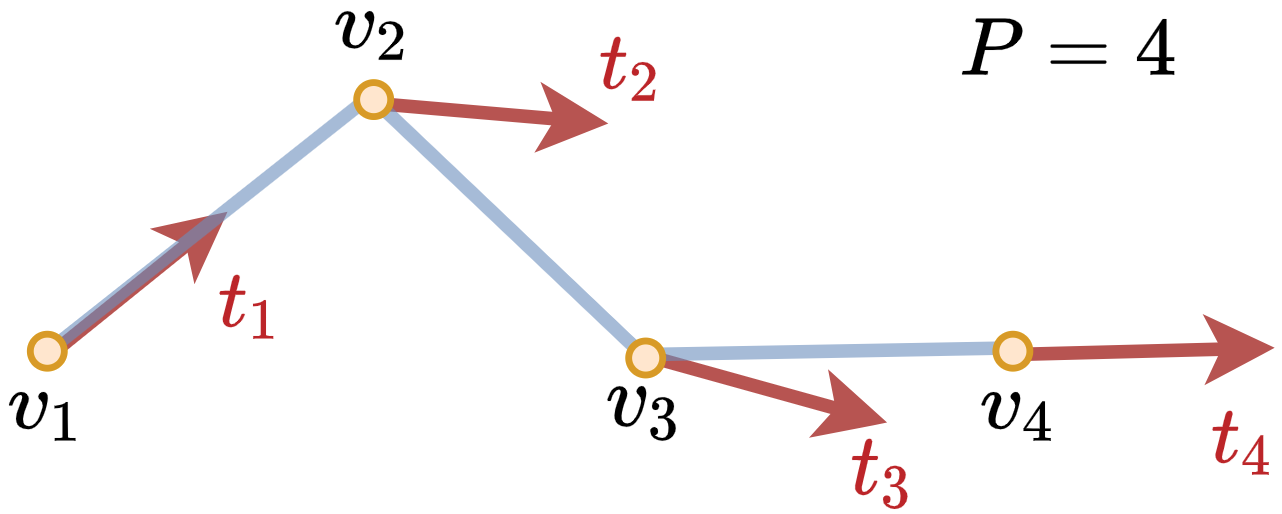
vecs_tan(curve, normalized=False)

Get the tangent vectors at points on a curve. Specifically, let \(t_i,1\leqslant i\leqslant P\), be the \(i\)-th tangent vector, and \(v_i\) be the \(i\)-th point. Then, \(t_1=v_2-v_1,t_P=v_P-v_{P-1}\), and for \(2\leqslant i \leqslant P-1\), \(t_i=\frac{v_{i+1}-v_i}{\|v_{i+1}-v_i\|}+\frac{v_i-v_{i-1}}{\|v_i-v_{i-1}\|}\). \(t_i\)'s can be further normalized to unit vectors, if normalized is True.

Parameters:

Name	Type	Description	Default
curve	ArrayLike	Shape of [P, 3] (\(P\geqslant 2\)), an array of 3D coordinates representing the points on the curve.	required
normalized	bool	If True, all tangent vectors are normalized to have unit length.	False

Returns:

Name	Type	Description
vecs	NDArray	Shape of [P, 3]. vecs[i, 3] is the 3D coordinates that represent the tangent vector at the i-th point.